Rethinking the True Run Value of a Pitch With a Pitch Model
By John Asel, Baseball Ops Intern
Our intrinsic pitch values combine stuff and pitch location to predict the expected change in run value a given pitch should create based on its raw flight characteristics. It is pretty darn good, but it is not perfect. Certain pitchers—through deception, sequencing, tunneling, etc—have demonstrated the ability to consistently exceed our expectations from year to year.
We know players like this will exist, but how much data do we need until we can confidently say that someone is an outlier relative to their peers?
That question is the basis of this investigation.
Methodology
The metric we will be using across these analyses is the change in run value (RE12 with an xwOBA base) minus the intrinsic pitch value (from our pitch model); in other words, the difference between the observed and expected run value changes on a pitch-by-pitch basis.
We’ll refer to this metric as “intrinsic residual” where negative is the pitcher performing better than expected.
To test the reliability of “intrinsic residual”, we will be using Cronbach’s alpha. For those unfamiliar with Cronbach’s alpha, FanGraphs wrote a great introduction in 2015 which we highly encourage you to read if you have not already.
The gist is that Cronbach’s alpha measures the internal consistency of a sample, giving us an estimate of what proportion of the variance observed is reproducible (likely due to ‘true talent’) as opposed to randomness. The typical alpha threshold considered reliable is 0.7—where ~50% of the variance is attributable to a rough proxy for ‘true talent’.
Player Level
With the gory math aside and our framework built out, we can first look at a player’s general intrinsic residual to give us a sense of the X factor they possess relative to our model.
A negative value indicates that a pitcher performed better than expected while a positive value indicates that a pitcher performed worse than expected. Taking the sum of these residuals on the pitch-by-pitch level can give us an idea which pitchers have cumulatively deviated from our model’s expectations the most during the Statcast era (2015-present).
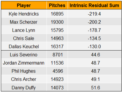
Keep in mind that the units of these residuals are runs. So, Kyle Hendricks has prevented 219 more runs over the Statcast era than our model predicted—even though the model does account for his otherworldly command.
To put that in perspective, according to baseballreference.com, Hendricks has prevented 126 runs relative to a league average pitcher. Without his X factor, our model thinks he would have been as below average as he has been above average.
Had Hendricks not possessed such an ability to exceed expectations, he would not be the pitcher he is today and he would not get the playing time he gets today. In other words, players with poor X factors are fighting an uphill battle because they must be several runs better to survive.
This is the essence of survivorship bias and it explains why the pitchers who are beating our model by the most are doing so at a higher magnitude than those who are relatively underperforming. For example, if a hypothetical pitcher had a X factor that hurt them as much as Scherzer’s X factor helps him, they would have to possess elite stuff just to be league average.
Then again, the analysis above is just taking the sum of residuals, which is highly dependent on playing time accrued. To avoid playing-time bias, we need to build a rate statistic and use some sample size threshold to find the true leaders and laggards.
That brings us back to the question we set out to answer: At what point can we be confident that the intrinsic residual we are observing is not just randomness?

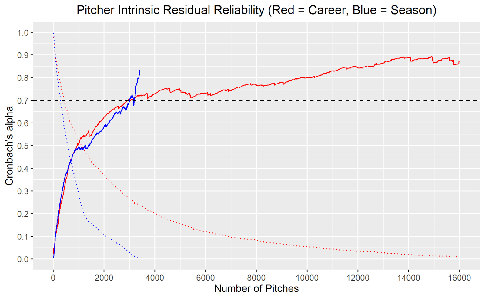
To answer this question, we need to look at the graphic above showing Cronbach’s alpha values at various sample sizes on the season (blue) and career (red) levels. It is a lot to look at if you have not seen one of these graphs before, so let’s do an example interpretation.
When X = 1000, the required sample size to be included is 1000 pitches thrown. Looking at the graph’s dotted lines, we see that ~50% of pitchers and ~30% of pitcher-seasons in the Statcast era have thrown 1000+ pitches. When those with less than 1000 pitches are filtered out of our sample, the alpha value is ~0.5 for both the season and career levels. Thus, we can infer that when looking at a player’s entire career or at a specific season, it takes approximately 1000 pitches for 25% of their average intrinsic residual to be explained by ‘true talent’ as opposed to randomness.
Example aside, we’re more concerned with the 0.7 threshold—the level where 50% of the variance is explained by ‘true talent’—and where it is crossed, as that is where most traditional baseball analysts consider a metric ‘reliable’. As shown above, this threshold is crossed just above 3000 pitches on both the season and career levels.
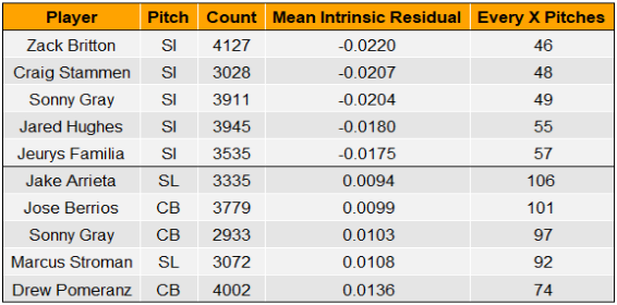
Below are the mean intrinsic residual leaders and laggards with a minimum of 3000 career pitches thrown in the Statcast era.
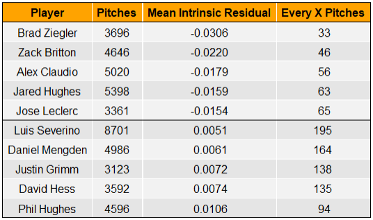
As in the previous table, we see that the pitcher-friendly residuals are of a larger absolute magnitude than the hitter-friendly residuals. Brad Ziegler, with his unorthodox release point, outperforms expectations by one run every 33 pitches!
Pitcher-Pitch Level
Looking at general X factors like this is cool, but how does it break down on the pitch type level? Do all pitchers’ pitches exceed expectations uniformly or do certain pitch types deliver the bulk of the benefits? Let’s run the same procedure but treat each pitcher’s pitch types distinctly.
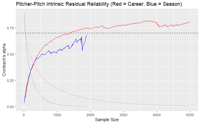
Grouping by pitch type cuts down on our sample size but is quite insightful. While players generally take 3040 pitches to reach career mean intrinsic residual reliability across all pitches, the average player-pitch type only takes 1400 pitches to do so. This suggests that, for any given pitcher, certain pitch types will systematically deviate from our model’s predictions to different degrees and—in some instances—in opposite directions.
An astute reader may be wondering, why do the season and career trends diverge around 400 pitches? Sample size is our friend here. What pitch types persist as the minimum sample size threshold is raised? Fastballs. If fastballs take longer to reliably defy our models, it makes sense for the slope of the Cronbach alpha chart to decrease as fastballs become a disproportionate part of the remaining pitch population.
To test this hypothesis, I looked at how long it takes each of the major pitch types to reach the alpha threshold of .7 at the career level.
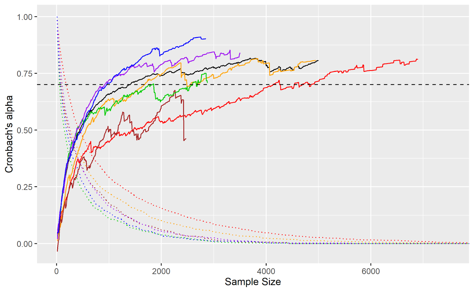
Figure Three: Red = Four-seamers, Orange = Sinkers, Green = Changeups, Blue = Curveballs, Purple = Sliders, Brown = Cutters, Black = All Pitch Types. The dotted lines pertain to the remaining proportion of that pitch type’s population that survives the corresponding sample size threshold.
As hypothesized, fastballs take longer to become reliable and come to dominate the population of remaining pitch types as the sample size threshold is raised. That explains the season-career gap in Figure Two, but let’s see what this graph has to say about the speed at which various pitch types become reliable.
| Pitch Type Bucket | Pitches to Reach Alpha = 0.7 |
| Four-Seamers | 4860 |
| Sinkers | 2550 |
| Changeups | 2690 |
| Curveballs | 960 |
| Sliders | 920 |
| Cutters | NA |
The intrinsic residuals of breaking balls reach the threshold far quicker than the other pitch types. This suggests a contextual nature to breaking balls. Whether due to arsenal interplay or a particular dependence on deception, the outcomes of sliders and curveballs relatively quickly diverge from what their raw flight characteristics would suggest.
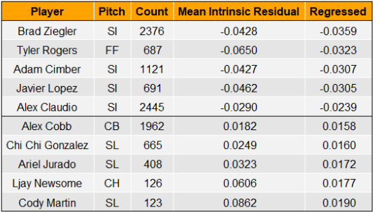
With these pitch-type-specific thresholds, we can see which pitches have reliably defied our model at both extremes.
In looking at the table above, we observe a lot of sinkers at the top, no? Indeed and there is quite a good reason for it: Seam-shifted wake (SSW).
We have written about this before, so to avoid rehashing too heavily, here’s the gist: When the seams on a pitch are oriented in a certain way, the ball will gain a particularly deceptive type of movement. This effect is most commonly observed in sinkers and those atop this list are known creators of this funky movement.
Our model, developed before SSW was discovered, looks at just the flight characteristics of a given pitch and cannot tell whether movement was produced normally or via SSW. With SSW being a key to a sinker’s success, it makes sense that many of the largest residuals come from those who generate the effect.
On the other end of the spectrum, we see all sliders and curveballs. It is interesting to note how elite these pitches are—maybe it is a clue to why breaking balls reach intrinsic residual reliability so quickly. Perhaps hitters know the quality of the pitch and must sit on it to some extent so they don’t end up on PitchingNinja.
That might be part of the reason Sonny Gray has two pitches on opposite ends of the spectrum; hitters are terrified of being embarrassed by his curveball and give up some extra ground to his sinker.
Regressed Pitch Values
After a certain number of pitches, we can be confident that a given pitcher’s pitch will continue defying our model’s expectations. But to what extent? At any given sample size, how much credit do we give the player? Thankfully, those Cronbach alpha values can help us out again. As detailed in a different FanGraphs article, the higher the alpha value, the less you regress to the mean.
So, in truth, there is no single point where you can suddenly start trusting the residuals. Instead, new data should be used in concert with what was already known to constantly refine our expectations going forward.
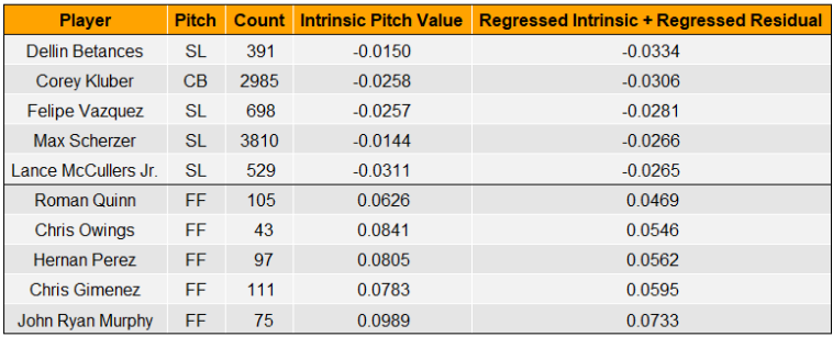
In the table above, we see some of the dirtiest breaking balls in the game at the top, with some position players at the bottom. Looking good.
That said, it is worth taking a moment to discuss how certain pitcher-pitch types end up at the top of this list. There are essentially three avenues that exist on a spectrum:
- Good intrinsic pitch value and large sample size of elite results
- Great intrinsic pitch value with results matching expectations
- Elite intrinsic pitch value with too small a sample size to prove the model wrong
The first avenue is well exemplified by the sliders of both Dellin Betances and Max Scherzer. Our model recognizes them as nasty pitches, but based on extraordinary results in sufficient sample sizes, our refined expectations rightfully elevate them to some of the best pitches in baseball.
Although Sam Clay’s slider falls just outside the top five pitches, it is a golden example of the third avenue: Underperforming yet ultimately rate highly. The key to such a feat? Pitch count.
At the time of writing, Sam Clay has thrown 149 sliders in the major leagues. That pitch count corresponds with a high intrinsic pitch value reliability (alpha = 0.88), but a low intrinsic residual reliability (alpha = 0.20). In simpler terms, we have a strong belief that Clay’s SL is nasty, even by lofty big-league standards, and we cannot be sure that it will continue to underperform our expectations moving forward due to a small sample size.
Pitches can still rate highly if the results on the field provide insufficient evidence to overrule the model’s original output.
The Application of Regressed Run Values
When evaluating an athlete, we need to understand which pitches are assets and which are ripe for improvement. Stuff+ from The Blob tells most of the story, but command and results need to be considered as well.
Imagine a pitcher with a changeup that grades below average in raw stuff, but who also has impeccable command with the pitch. If they could adopt a better shape with the same feel, that would be great, but there is likely lower hanging fruit in the arsenal. Further, if the changeup has consistently produced better results than expected, we can be confident that it is not in need of fixing.
Getting better starts when building a plan of attack; finding weaknesses and ways to improve them. With this infrastructure to weigh in-game success against raw flight characteristics, we can decode mixed signals and better aid the outliers on their path to greener pastures.
Comment section